Tracking Donations using Google Sheets
I organize an annual fundraiser for the Multiple Myeloma Research Foundation (MMRF). Multiple myeloma is the second most common blood cancer and there is no cure. When my mom was diagnosed with it in 2010, the life expectancy was just 36 months. It’s extraordinarily rough to hear that kind of news, especially when you are an otherwise young and healthy adult. When she passed away in May of 2014, I knew I had to do something to help other families dealing with MM. I started up Play It Forward as a way to honor and remember her as well as raise money and awareness for MM. The fundraiser is sort of unique in that participants pay an admission fee ($10) to come play board games with other people. My boyfriend and I supply a few hundred games to choose from and some people bring their own as well. In it’s first year, we raised over $4,200. I think I will always look back at that event as one of my proudest moments. While the first year was a success, there were still many bumps along the way. I had my sister run the check in desk and I wanted her to track all of the money she was receiving, what it was for, who it was from, etc. I made a Google Sheets spreadsheet which made sense to me but, as it turned out, didn’t make sense to her. She ended up trying to make it easier to understand for herself but in the process messed up a lot of the formulas I had put in place. I want to spend a little bit more time designing a form and spreadsheet to track the money coming in for this year’s event (which is in just a few days, on December 12, 2015). I want it to be done in a way that is really intuitive so that whoever is at the check in desk at the time can get the job done correctly, but I also need to get it set up in short amount of time.
Google Forms
I could make a MySQL database with a corresponding VB GUI but I don’t want to run the risk of running into a programming issue at the event. What I’m wanting to track is fairly straightforward, so Google Forms should work out just fine. To start a new Google Form, simply go to drive.google.com and click on the red ‘NEW’ button on the left. In the drop down, click ‘Google Form’ (you may have to click ‘More’ to get it to show up). Designing the form is very straightforward. You can mark questions as mandatory and you can do simple data validation such as making sure the text entered is a number or a number in a specific range. It didn’t take very long for me to come up with a form that looks like this: 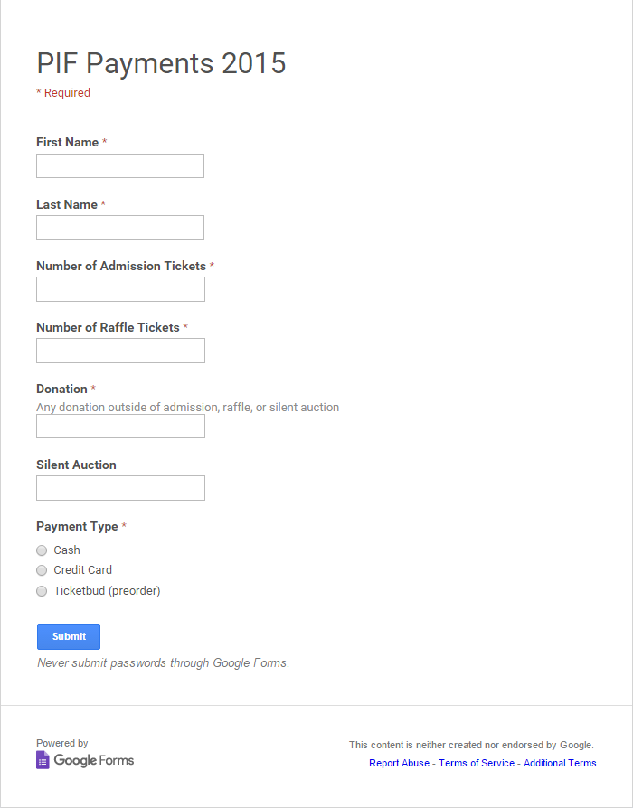 Every field except for Silent Auction is mandatory (this is because the silent auction will be held later in the day and only a few people will actually win items). First and last names need to be text, while the rest of the fields must be numbers equal to or greater than zero. Finally, the payment type is a radio button choice (the user can only choose one type). Once you press submit, the information gets put into a spreadsheet called ‘PIF PAYMENTS 2015 (Responses)’. The biggest thing I’ve learned from using Google Forms is that you always leave your raw data sheet alone. Do not do calculations or manipulations on that sheet, do them in another! The first sheet, ‘Form Responses 1’ has the following columns:
- Timestamp
- First Name
- Last Name
- Number of Admission Tickets
- Number of Raffle Tickets
- Donation
- Payment Type
- Silent Auction (this is last because I added it to the form last, even though it isn’t last on the form)
The data in this sheet comes directly from the form and is my raw data sheet.
Transaction Summary Sheet
Next, I have a sheet titled Transaction Summary. This takes each transaction from the Form Responses 1 page and calculates how much money that person spent on their transaction. The different items and their costs are:
- Admission: $10
- Raffle Ticket: one ticket for $3 or four for $10
In addition to tickets, people may donate money or pay for their silent auction items as well. These categories could be of any amount. The ‘Transaction Summary’ sheet has the following columns:
- Date
- First Name
- Last Name
- Type (options are Cash, Credit Card, or Ticketbud (which is used for preorders))
- $ Admission
- $ Raffle
- $ Auction
- $ Donation
- Transaction Total
- Total Raffles
 The first four columns are pulled directly from the Form Responses 1 spreadsheet. However, when you submit an entry using Google Forms, Google will insert that data as a new row. This means I can’t simply put the formula [text] =’Form Responses 1’!A2 [/text] into cell A2 of Transaction Summary and click and drag it down. Say you have five responses in your spreadsheet already (therefore you have had five transactions and there are 6 rows in both the Form Responses 1 and the Transaction Summary spreadsheets). If you had simply done the ‘click and drag’ method on the formula above then the next empty cell in column A, cell A7, would have the formula [text] =’Form Responses 1’!A7 [/text] This is great if you are simply adding information to row 7 in the Form Responses 1 sheet. However, since Google inserts a row when it submits the data from its form, all of your references in other sheets will be moved down one row. This means the cell that once said [text] =’Form Responses 1’!A7 [/text] now incorrectly says [text] =’Form Responses 1’!A8 [/text] To fix this, we use the *ARRAYFORMULA *function.
ARRAYFORMULA
The ARRAYFORMULA function within Google Sheets is another extremely powerful function (I discussed perhaps the most powerful Sheets function, FILTER, here). It allows you to manipulate an entire column by only filling in one cell. This is what we need because we don’t want to have to reference back to the raw data sheet on a cell by cell basis since we know every time data gets entered, our reference will be thrown off. Our new function in cell A2 of Transaction Summary should then be: [text] =ARRAYFORMULA(‘Form Responses 1’!A2:A) [/text] ARRAYFORMULA requires at least one cell range, which is why I changed A2 to A2:A (I could also give it a limit, such as A2:A500 and this would save memory and efficiency). ARRAYFORMULA also requires empty cells below the cell you enter the formula in because it wants to fill in these cells with data. If the cells are not empty, you will receive a #REF! error. The next three columns, First Name, Last Name, and Type are done in the same way. [text] =ARRAYFORMULA(‘Form Responses 1’!B2:B) [/text] The last several columns calculate how much money is spent in the different available categories. Admission is a flat rate of $10, so the formula for that column is quite simple: [text] =ARRAYFORMULA(‘Form Responses 1’!D2:D * 10) [/text] Where column D is the number of admission tickets purchased (which we get from the form submission). Next is the money spent on raffle tickets. This is a little trickier because the raffle tickets are not a flat rate. The tickets are $3 each but if you buy 4 they are only $10 (instead of $12). In order to figure out how much money a certain number of tickets cost, we must first understand the MOD function.
MOD
The MOD function gives the result of the modulo operator. In other words, it gives the remainder after a division operator. The arguments within MOD are MOD(dividend, divisor). For example, MOD(8,4) would be 0 because 4 divides into 8 evenly, with no remainder. However, MOD(9,4) would be 1 because 1 is the remainder of 9/4. If a person purchased raffle tickets in a multiple of 4, then MOD(number of tickets purchased, 4) would be equal to zero. In this case, the cost for the tickets is simply [text] $10 * Number of tickets sold / 4 [/text] If a person didn’t buy the raffle tickets in a multiple of 4, that doesn’t mean they didn’t buy any tickets in a multiple of 4. For instance, if you purchased 10 tickets, the previous check would say you didn’t buy any tickets in a group of 4. This is because MOD(10,4) = 2 and not zero as we had above. However, if you purchased 10 tickets you actually purchased 2 groups of 4 with an additional 2 individual tickets. To check for this case, we round down the result of [text] number of tickets / 4 [/text] In this case, rounding down 10/4 gives 2. We must add that to the remainder, which we get from the MOD function. All told, the formula would look like: [text] $10 * floor(number of tickets/4) + $3 * mod(number of tickets,4) [/text] In order to incorporate this into my spreadsheet, I need to wrap it in a few if statements and make it compatible with the ARRAYFORMULA function. The final formula looks rough but it gets the job done: [text] =ARRAYFORMULA(IF(‘Form Responses 1’!E2:E>0,if(mod(‘Form Responses 1’!E2:E,4)=0,10‘Form Responses 1’!E2:E/4,if(mod(‘Form Responses 1’!E2:E,4)>0,floor(‘Form Responses 1’!E2:E/4)\10+mod(‘Form Responses 1’!E2:E,4)*3)),0)) [/text] The following two columns, $ Auction and $ Donation, are done in the same way as the first column was done (with the ARRAYFORMULA). Transaction Total calculates the total amount of money a person is donating through his or her purchase of admission and/or raffle tickets, silent auction, and donations. This is simply the sum of the four previous columns ($ Admission, $ Raffle, $ Auction, and $ Donation). However, we again want to put this into ARRAYFORMULA so that when data is entered into the Form Responses 1, the references won’t get misaligned. The formula for this may not be intuitive: [text] =ARRAYFORMULA(G2:G + H2:H + I2:I + J2:J) [/text] For each row, this will sum columns G through J, giving the total donated for each transaction. The final column, N, counts how many raffle tickets a person should receive at the door. If the person purchased tickets before a week prior to the event, they receive a free raffle entry. The formula for this simply looks at the total number of raffle tickets (which is given through the form), and adds one if the date is before the week before the event. [text] =ARRAYFORMULA(‘Form Responses 1’!E2:E + if(A2:A < date(2015,12,5),1)) [/text]
Donor Summary Sheet
I want to track how much money each person donates through the fundraiser but each person may donate through multiple transactions. For instance, many people purchase their admission tickets ahead of time but they may win an item at the silent auction and need to pay for it at the event. Or, they could see that the raffle prize is growing large and decide at the event to purchase additional raffle tickets. I wanted a sheet that looks at each unique first/last name combination and gets a sum of all of their donations. Prior to learning about database design and optimization, this problem would have really stumped me. However, working with databases has allowed me to think about problems like this in a different light. The ‘Donor Summary’ sheet has the following columns:
- Name (this is full name)
- Admission Tix (number of tickets)
- Paid Raffle Tix
- Free Raffle Tix
- Auction
- Donation
- Total
I needed something like a primary key for each individual at my event so that I could track things about them such as how many of each ticket type they get and ultimately how much they donated. I decided the chances of multiple people having the same first and last name attend my event were slim enough that I would make each attendee’s full name their ‘primary key’. The first column, Name, gets a list of all of the unique full names from the raw data sheet. This is pretty simple: [text] =unique(ARRAYFORMULA(‘Form Responses 1’!B2:b&” “&’Form Responses 1’!C2:C)) [/text] Form Responses 1 column B is first name and column C is last name for each transaction. The ampersand (‘&’) concatenates things on either side of it (with seemingly no limit. The ‘CONCAT’ function will only take two arguments so to get around this, use ‘&’ instead). Finally, the ‘unique’ command only shows each response once. The rest of the columns are all very similar. To figure out the total number of admission tickets a person purchased, even if they were over multiple transactions, I use the formula: [text] =sum(filter(‘Form Responses 1’!$D$2:D, ‘Form Responses 1’!$B$2:B &” “&’Form Responses 1’!$C$2:C = A2)) [/text] This function looks a little intimidating at first. Long spreadsheet formulas are generally best understood starting at the center and working out. Here, we first use the ‘filter’ function. We want to get the values from Form Responses 1 column D which are the number of admission tickets (which is from the form) where the concatenation of the first name and last name equals the unique name in column A2. This may result in several rows of values, so we sum everything. A critical part of this function are the dollar signs on either side of the ranges. We will use the click and drag method for this function, meaning we will drag this function down the spreadsheet to copy the formula. We want to always consider all of columns D, B, and C so we need to put the dollar signs on both sides of those column declarations (otherwise, when you drag the formula down it would change from D2:D to D3:D, D4:D, etc). We want the A2 reference to change based on column so that we continue to look for the next person in the column.
Payment Type Sheets
The last sheet that I currently have is the Payment Type sheet. There are a few ways people could donate to the cause or purchase tickets: cash/check, credit card, or online (through Ticketbud). Cash and check come to no cost to me. However, the credit card processing company I use charges a fee based on swipe and the online ticketing system charges based on ticket sold. I have committed to making sure that 100% of the money people donate to my fundraiser actually goes to the MMRF. Because of this, I’ve committed to covering 100% of the fees that the credit card and ticketing system deduct. Since I’m paying for this, I want to track these costs that I will bare. The Payment type spreadsheet is intended to help me see this. It has the columns:
- Date
- First Name
- Last Name
- Payment Type
- # Admission Tickets
- # Single Raffle
- # Group Raffle
- Donation
- Auction
- PIF Cost
Many of these columns are the same as what we have previously discussed. The most interesting and most complicated is the last column, PIF Cost. A summary of my costs based on transaction type is below:
- Ticketbud
- $1.33 per admission ticket
- $1.06 per single raffle ticket
- $1.33 per group raffle
- Credit Card
- 2.7%
- Cash/check
- No cost
In order to get the sum per transaction of the cost to me, the formula is: [text] =ARRAYFORMULA(if(E2:E=”Ticketbud (preorder)”,1.33*F2:F+1.06*G2+1.33*H2:H,if(E2:E=”Credit Card”,’Transaction Summary’!L2:L*0.0275,if(E2:E=”Cash”,0,”Payment Type?”)))) [/text] This formula checks if the payment type is Ticketbud. If it is, it simply multiples the number of admission tickets and group raffle tickets by $1.33 and the number of single tickets by $1.06. People cannot pay for donations or auction items through this service, so I don’t have to worry about it. It then checks if the payment type is credit card. If it is, it simply takes their total and multiples it by the 2.75%. I’m sure I will add more sheets to this spreadsheet before the event is completely said and done but the majority of its final functionality is there and with relatively little work. I would like to add two large cells, perhaps in a new sheet, that give the most recent transaction total and total raffles. This way, whoever is running the front desk can easily see how much an attendee owes and they will hopefully not have to do very much math.