Machine Learning Part 2: Visualizing a Decision Tree

Google released their second video on machine learning last week. It is titled Visualizing a Decision Tree - Machine Learning Recipes #2. If you missed my overview of the first video, you can check that out here. In this post, we will build a decision tree from a real data set, visualize it, and practice reading it.

Types of Classifiers

In our last post, we used a decision tree as our classifier. With that project, we used the classifier to distinguish between apples and oranges based on weight and texture. Decision trees aren’t the only type of classifiers – other types include artificial neural networks () and support vector machines. Decision trees are unique because they are easy to read and understand – we can understand exactly why a classifier makes a decision because we can literally see the questions that the classifier makes and asks in order to come to its conclusions.

Iris Flower Data Set

In this post, we’ll be working with the Iris data set (the Wikipedia page has a lot of information, including all of the data) - this is a real data set and a classic machine learning problem. This data set is also known as Fisher’s Iris data set and Anderson’s Iris data set. The data set is a total of 150 samples of different species of Iris – 50 samples each for Iris setosa, Iris virginica, and Iris versicolor, each of these are pictured above. For each sample, researchers collected the length and width of the sepals and petals (so, 4 measurements per sample). Our goals will be similar to our last post. We want to import the data set into Python, Train a classifier, Predict the flower based on new measurements, and finally, Visualize the tree.

Import The Data Set

We will be using scikit-learn again for this problem. Scikit-learn has 5 data sets built in that we can easily import. Luckily for us, the 150 samples for the Iris data set is included. To import the data set, start a new Python script: [python] from sklearn.datasets import load_iris iris = load_iris() [/python] This data set includes the 5 columns and 150 rows of data that we can see in the Wikipedia article as well as some metadata. For example, we can see the features by using: [python] print iris.feature_names [/python] Remember, features are the qualities that we measured to classify our data. The output of this command is: [text] [‘sepal length (cm)’, ‘sepal width (cm)’, ‘petal length (cm)’, ‘petal width (cm)’] [/text] We can see the targets by using a similar command: [python] print iris.target_names [/python] The result here are the outputs that we expect (known as the targets): [text] [‘setosa’ ‘versicolor’ ‘virginica’] [/text] The actual measurements are stored in the data object. To see the actual numbers for a specific measurement, we can use: [python] print iris.data[0] [/python] This will give: [text] [ 5.1 3.5 1.4 0.2] [/text] These numbers correspond to the sepal length, sepal width, petal length, and petal width in centimeters respectively. In fact, if we check the table on Wikipedia, we see that these numbers match exactly! 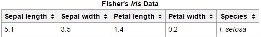As we would expect, the target object contains the labels. To see which flower was measured for each test, we can use: [python] print iris.target[0] [/python] In this case, we expect the output to be setosa (we can see from the actual data above that these measurements belong to the setosa species). The output is maybe not what you expect: 0! However, these outputs correspond to the targets from the iris.target_names variable. Therefore, a label of 0 corresponds to setosa, 1 corresponds to versicolor, and 2 corresponds to virginica.

Train the Classifier

Now that we understand the data and can work with it a little, we need to train our classifier. First, we want to split up the data. With our 150 samples, we want to use some as training data and some as testing data. Training data will be used to train our classifier and the testing data will be used to check to make sure our classifier works properly. We want to separate the data so that the testing data will be new to the classifier. The data set is ordered such that the first entry is a setosa, the 50th is a versicolor, and the 100th is a virginica. We will remove each of these and use them later to test our data. [python] import numpy as np from sklearn.datasets import load_iris iris = load_iris() test_idx = [0, 50, 100] train_target = np.delete(iris.target, test_idx) train_data = np.delete(iris.data, test_idx, axis=0) test_target = iris.target[test_idx] test_data = iris.data[test_idx] [/python] Here, I created a variable, test_idx, which is the index (or location) of one of each type of flower. Next, we create our training targets (the labels, or what type of flower) and our training data (the actual measurements). The np.delete command has two inputs: the first is the all of the data and the second is a list of the locations of the data you want to remove. For our training target data, we want to take all of our training targets (iris.target) and remove the rows in the data that correspond to the 0, 50, and 100 index locations (which is stored in the test_idx variable). For the training data, notice that the input includes an addition attribute: axis=0. This is because the training data is a list of lists. In other words, if we print the training data, it would look similar to this: [text] [[ 5.1 3.5 1.4 0.2] [ 4.9 3. 1.4 0.2] [ 4.7 3.2 1.3 0.2] [ 4.6 3.1 1.5 0.2] [ 5. 3.6 1.4 0.2] …..] [/text] The axis=0 attribute tells Python to delete an entire row of data. In a simple list, such as that of the training targets, a location of 0 can mean only one thing so the additional attribute is not needed. Next, we create our testing targets and testing data. We do this by simply inputting our desired indices into the target and data variables.

Predict

We can do a test to make sure part of this worked by printing the test_target variable: [python] print test_target [/python] Since we specifically chose 0, 50, and 100 to be one of each type of flower, we expect the output of this to be [0 1 2]. When we run it, the output is what we expect. Finally, we can train our classifier. We do this just like we did in the last post (be sure to put from sklearn import tree at the top of your script): [python] clf = tree.DecisionTreeClassifier() clf.fit(train_data, train_target) [/python] Now, we can use our testing data to see if the script correctly predicts our flowers. Remember, the output we expect is one of each (in other words, we expect an output of [0 1 2]). [python] print clf.predict(test_data) [/python] This results in the correct output: [0 1 2]. This means the script got everything correctly!

Visualize the Tree

Scikit-learn has some great tutorials on their website. To visualize the tree, we combine code from a couple of different tutorials to come up with: [python] from sklearn.externals.six import StringIO import pydot dot_data = StringIO() tree.export_graphviz(clf, out_file=dot_data, feature_names=iris.feature_names, class_names=iris.target_names, filled=True, rounded=True, special_characters=True) graph = pydot.graph_from_dot_data(dot_data.getvalue()) graph.write_pdf(“iris.pdf”) [/python] I am using Python 2.7 and when running this code, I came across an error: [text] NameError: global name ‘dot_parser’ is not defined [/text] The solution for me was to install pydotplus and replace pydot with pydotplus in the code. The pdf output looks like this: 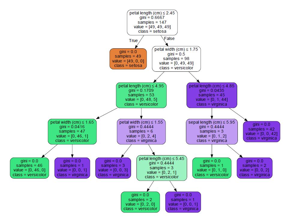We read decision trees much like a flow chart. Boxes with arrows leading out of them are questions. If the answer is true, you take the left arrow. If the answer is false, you take the right. Boxes at the end (without any arrows out of them) are the predictions. Lets take the following data and follow it through the tree (I just grabbed a random row from the table on Wikipedia): [table width=”500” colalign=”left|left|center|left|right”] sepal length, sepal width, petal length, petal width, species 7.7, 2.6, 6.9, 2.3, virginica [/table] The first question is: Is the petal length less than or equal to 2.45 cm? Our petal length is 6.9 cm, so the answer to this question is false - we move to the right. Next, petal width less than or equal to 1.75 cm? Our petal width is 2.3 cm. Again, the answer is false so we move right. Is the petal length less than or equal to 4.85 cm? Our petal length is greater than that (6.9) so we move to the right. This box has no arrows coming out, so we are at a prediction. The bottom of the box lists the prediction: class = virginica – it got it right! Below is an image of the path we took to get to our prediction.

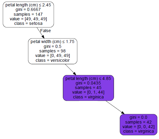
Final Thoughts

You can grab a copy of my code on my gist here. This project was really fun for me. I love using real data and it is absolutely mind boggling to me that Python is able to generate this decision tree. The fact that it does it so quickly is also really amazing to me. I can’t wait to learn more about what is going on behind the scenes and to use this for some of my own projects. Have questions or suggestions? Please feel free to comment below or contact me.